Decision Trees: The First Step Toward Ensemble Learning

Today, the forefront of machine learning and data science is dominated by large language models (LLMs), multi-agent systems, and deep neural networks. Despite their power and widespread use, traditional, simple, and well-interpretable predictive models remain extremely important for business. Decision trees, which form the foundation of one of the most effective algorithms for tabular data — XGBoost — are a prime example of how classical machine learning models lay the groundwork for the further development of artificial intelligence.

Understanding this fundamental algorithm allows us to apply a whole range of ensemble models more effectively and accurately to solve many critical business problems, such as demand forecasting or medical classification. For this reason, we decided to launch a series of posts where we will clearly and thoroughly explain the core principles of modern machine learning. And today, we begin with Decision Trees.

Brief Historical Overview

Decision trees have their roots in early statistical classification and decision-making research. Their development spans several fields—statistics, psychology, operations research, and later, artificial intelligence and machine learning.

Early forms of decision trees were developed in statistics for classification and prediction. A key milestone was the introduction of AID (Automatic Interaction Detection) by Morgan & Sonquist (1963), one of the first algorithms to generate classification trees.

In the time period between 1975–1993 appeared more sophisticated tree-building methods:

• CART (Classification and Regression Trees) by Breiman et al. (1984) established the modern framework for both classification and regression trees.
• ID3 by Quinlan (1986) introduced entropy and information-gain-based splitting and helped popularize decision trees in artificial intelligence.
• C4.5, introduced in 1993, improved ID3 by adding support for continuous features, applying pruning techniques, and becoming more robust overall.

During the 90s, decision trees became a standard method in machine learning due to their interpretability and strong predictive performance. In the 2000s they evolved into the basis of powerful ensemble methods such as:

• Random Forests (Breiman, 2001)
• Gradient Boosting Machines (GBM)
• XGBoost, LightGBM, CatBoost

These methods combine multiple trees to achieve higher accuracy and robustness, making them central to modern machine learning and data science.

Definition

Decision trees can learn patterns from data by recursively splitting features. They not only provides interpretable decision rules, but also serve as the foundation for many high-performing ensemble approaches. Nowaday, they remain widely used for classification, regression, feature importance analysis, and decision support systems.

By definition, decision tree is a predictive model that organizes decisions and their possible outcomes in the form of a branching, tree-like structure. Each internal node represents a question or condition based on a feature, each branch shows the result of that condition, and each leaf node represents a final prediction or decision. It works step-by-step, splitting data into smaller, more uniform groups, making it intuitive to interpret and visualize. In essence, a decision tree mimics human decision-making: start with a question, follow the answer branch, and continue until you reach a conclusion.

Every day, we make choices — often without even realizing it. For example, we decide what to wear based on the weather, or choose what to eat by thinking about what we like and what is available. We naturally follow a step-by-step process: we ask ourselves questions, consider the answers, and then take action.

A Decision Tree works in a similar way. Just like we ask questions to guide our choices, a decision tree asks questions to reach a final decision. It helps machines think through possibilities one step at a time, branching out based on answers until it finds the best conclusion.

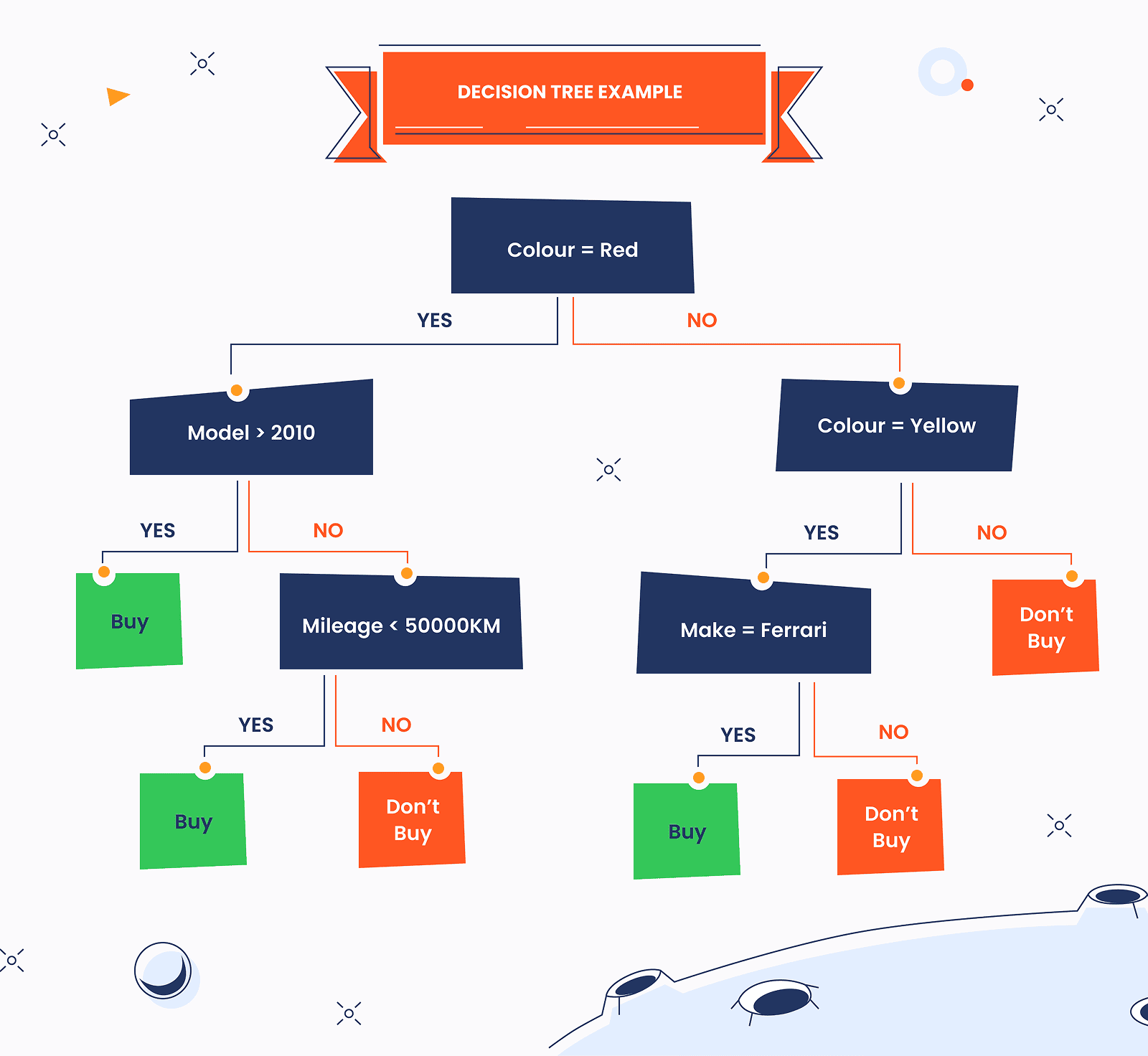
Source: Iglesias, Martin. (2021). Dimensional and Discrete Emotion Recognition using Multi-task Learning from Acoustic and Linguistic features extracted from Speech.

In the visual example, the decision tree begins with the root node — labeled Colour — which represents the top-level decision point. From this node, the decision splits into two possible paths based on the attribute value.

It is common practice for the Yes branch to extend to the left and the No branch to extend to the right. As we follow these branches, we encounter additional internal nodes that continue to divide the decision process using other features.

Eventually, the traversal reaches the terminal (leaf) nodes, which contain the final outcomes. These leaf nodes represent the end of the decision path and provide the resulting classification or decision.

A decision tree typically consists of nodes and edges, structured as follows:

• Root node — the topmost node, representing the initial decision point.
• Internal (split) nodes — nodes that have children and represent tests or features used to divide the data into subgroups.
• Leaf or terminal nodes — nodes without children, representing the final outcome or decision.
• Edges (branches) — connections between nodes that represent the flow or decision path from one node to another.

Building the Decision Tree (CART)

In provided explanatory materials we will consider CART paradigm as the classical and most simple approach. Variations of trees like ID3 and C4.5 utilize slightly different techniques for building the decision processes, thus we will not describe them here.

CART stands for Classification and Regression Trees. This approach produces only the binary trees, i.e., it always splits nodes into two children (left/right). Also, CART uses different impurity criteria depending on the task: Gini impurity for classification and mean-squared error (MSE) or mean absolute error for regression (we will cover this in the sections below). It can handle both numerical and categorical features and performs post-pruning to avoid over-fitting (finds a sequence of pruned subtrees and chooses the best with cross-validation dataset).

To understand how a CART based decision tree is constructed, let’s walk through a simple example.

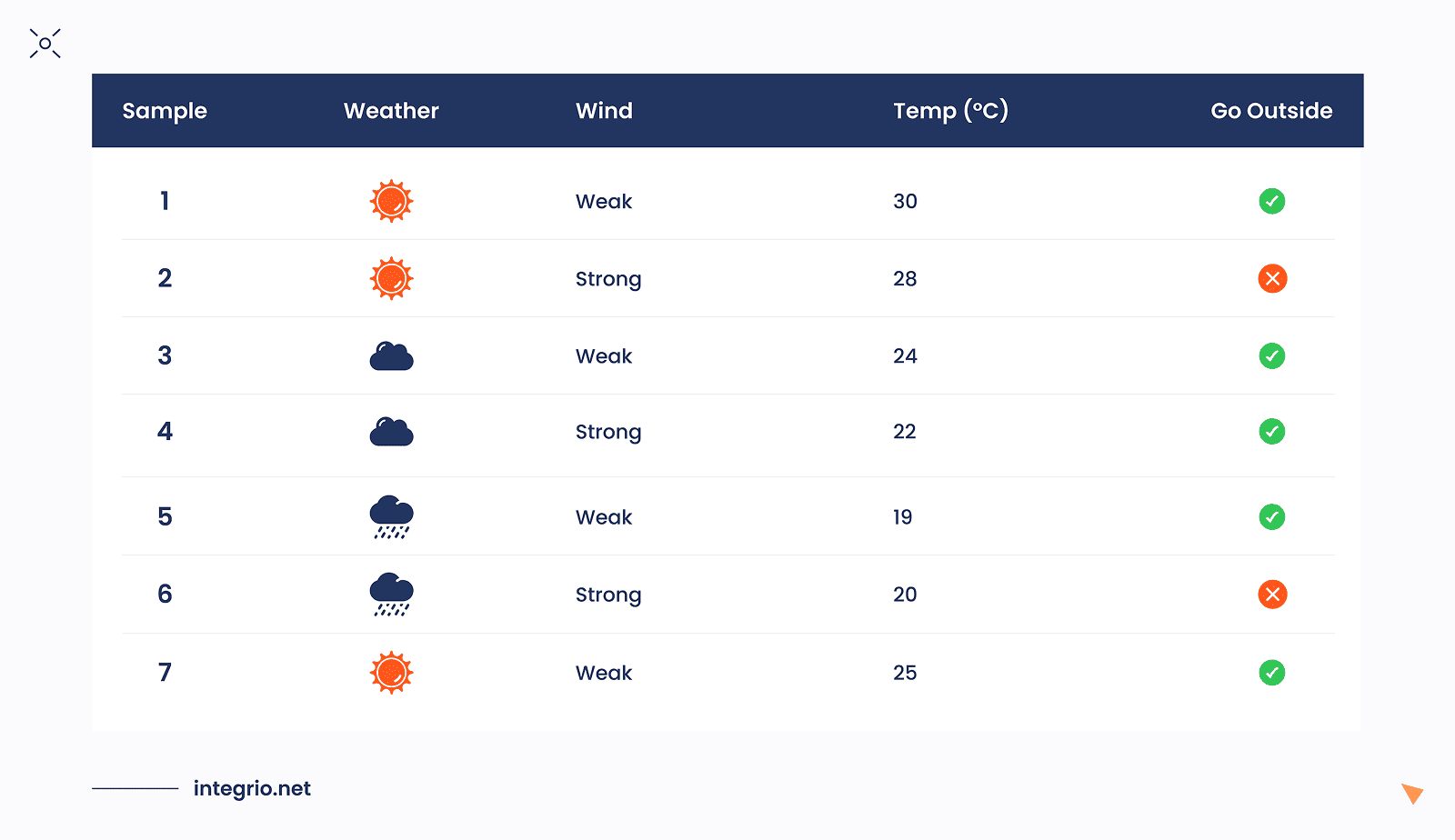
Assume we have a small weather dataset containing several input parameters — also referred to as features in machine learning. The weather conditions are represented using categorical variables: Weather {Sunny, Cloudy, Rainy}, Wind {Weak, Strong}, and a continuous feature Temp with values in the range [18, 30].

Our target variable, Go Outside, is a binary label with two possible outcomes: {Yes, No}. What we want is to build the classification tree model which will predict the target variable based on the combination of features. If the target is continuous variable, then we get a regression tree, another special type of decision tree.

The dataset below (Table 1) will be used to illustrate how the model learns decision rules from these features.

Processing Features/Nodes

Note, that here we have both categorical and continuous variables. Can we mix them together in Decision Tree? Absolutely! Below we will see how to make it properly.

To build a decision tree from the dataset above, the first task is to determine which feature should serve as the root node. The root should be the feature that most effectively splits the data according to the target label Go Outside. In other words, we want the feature that best separates Yes and No outcomes.

We have three candidate features:

• Weather
• Wind
• Temp

A simple way to begin with is to take one feature — for example, Weather — and evaluate how well it predicts the label Go Outside. This is our first splitting trial.

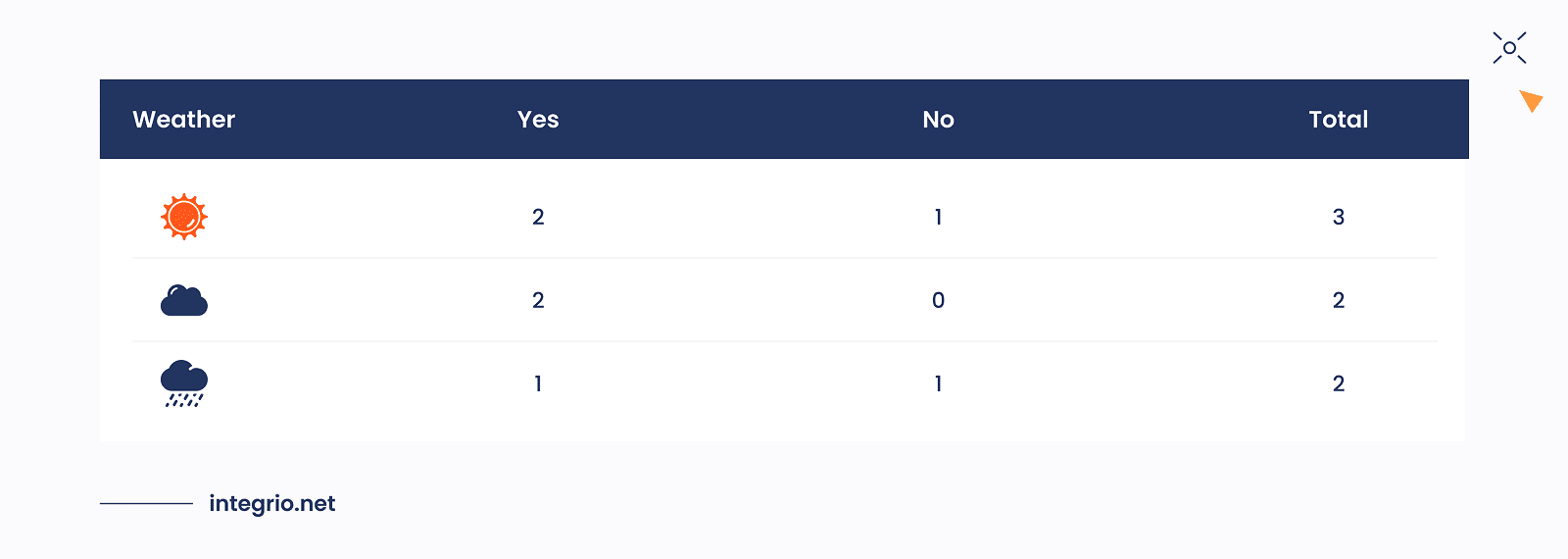
For each Weather values we can calculate a simple table of how much Yes and No labels are there for each feature value.

The same we can do with Wind feature.

Decision trees naturally handle categorical features, where a feature can be split based on equality (e.g., Weather = Sunny). But what about continuous (numeric) features like Temp?

We need a way to split numeric features into two groups: "less than a threshold" and "greater than or equal to a threshold."

Thresholding is a trick to convert a continuous feature into binary splits. Here’s how it works:

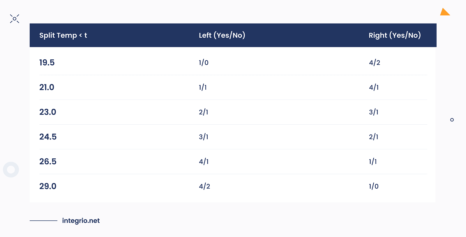
We sort the Temp values in ascending order: [19, 20, 22, 24, 25, 28, 30] and then compute midpoints between consecutive values to generate candidate thresholds: [19.5, 21, 23, 24.5, 26.5, 29].

Then, for each threshold we count the number of Yes and No labels as "<19.5", "<21", "<23", etc.

For instance,

Temp < 21 → [19, 20] → Labels = [Yes, No]

Temp ≥ 21 → [22, 24, 25, 28, 30] → Labels = [Yes, Yes, Yes, Yes, No]

This is the typical technique in CART classifier, which allows to process continuous features.

Splitting the Tree

By looking at obtained tables we can see rows like

and

These rows represents pure leaves, while all other are marked as impure leaves. This concept is very important in decision trees, because it describes the uncertainty of decision.

If a leaf provides a clear decision, meaning all instances in the leaf belong to the same class, there is no ambiguity about the outcome. In this case, we can be more confident that the label is fully determined by the splitting conditions that led to that leaf.

At first glance, it may seem that all features are equally effective at predicting the target whenever the resulting leaves are pure. While purity indicates that a feature contributes to separating the classes, relying solely on this qualitative observation is insufficient.

To objectively compare features and determine which provides the most effective splits, we need quantitative measures of uncertainty reduction. One fundamental concept in this context is entropy, which measures the disorder or unpredictability in a set of instances.

Decision tree algorithms like ID3 and C4.5 use entropy to compute Information Gain, which quantifies how much a feature reduces uncertainty when used to split the data. In the pure CART implementations Gini Index is set by default. By applying these metrics—especially those derived from entropy — we can systematically identify the best feature for splitting, rather than relying on intuition or apparent purity alone.

To calculate Gini Index for the node i there is a formulae:

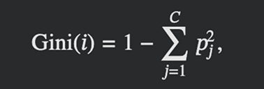
Where C is the number of classes and 𝑝_j is the proportion of instances in class j at that node. In other words, it is the probability of randomly picking two instances of different classes from node i. This formula comes from joint probability theory, which can be interpreted as follows: let 𝑝_j be the fraction of instances of class j in the node. Then:

• Probability that two randomly picked instances are of the same class j:
  
• Probability that two randomly picked instances are of the same class (any class):
  
• Probability that two randomly picked instances are of different classes

Interpretation:

• Pure node: p_j = 1 for some class j ⇒ Gini = 0
• Completely mixed node (for 2 classes): p₁ = p₂ = 0.5 ⇒ Gini = 0.5

Now, let's calculate Gini Indices for all our nodes: Weather, Wind and Temp.

For Weather feature we have three values: Sunny, Cloudy and Rainy. The numbers of samples for each of these feature values are presented in the table below.

The calculation of Gini Indices for this feature which is represented as nodes/leaves can be done as follows:

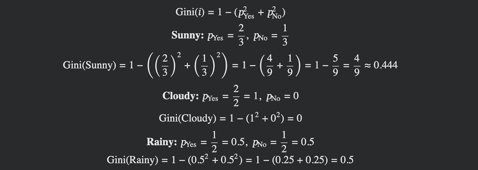
Because each leaf does not represent same number of samples: 3, 2 and 2 respectively, total Gini Impurity is the weighted average of the leaf impurities. This defined the weighted Gini for split value is:

For the Wind feature there are two leaves: Weak and Strong.

Weighted Gini for split is:

The calculation of Gini Indices and weighted Gini values for Temp feature involves a bunch of redundant computations.

Below are the results of these computations performed for each node.

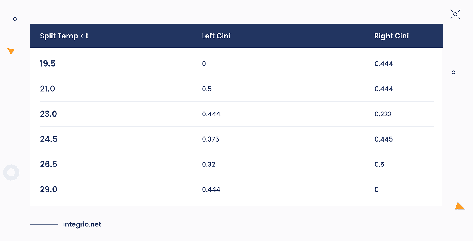
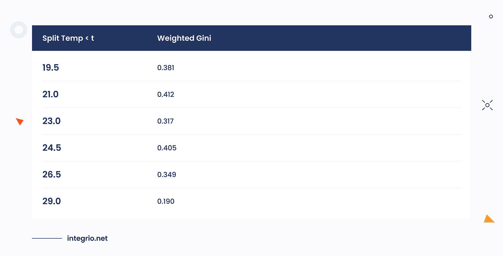
The aggregated results of all weighted Gini values for all leaves are gathered in the table below:

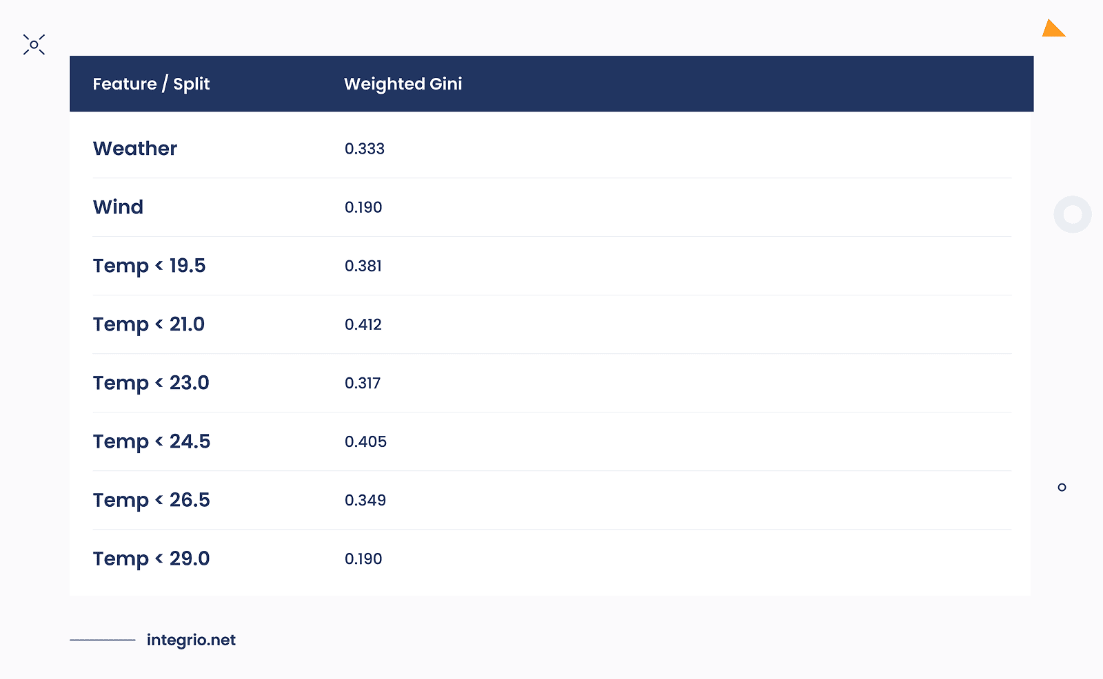
Lowest Gini index overall equals to 0.190. This occurs for Wind split: Weak / Strong and Temp < 29.0 split. Both splits produce subsets with high purity.

The decision tree algorithm can choose either feature. Typically, categorical splits like Wind are preferred first because they create clean separations without relying on numeric thresholds, but either is valid.

Both produce low impurity, but Wind is simpler and perfectly separates one pure leaf Weak → all Yes. This shows how Gini index quantitatively guides feature selection and identifies splits that produce the most certain (pure) leaves.

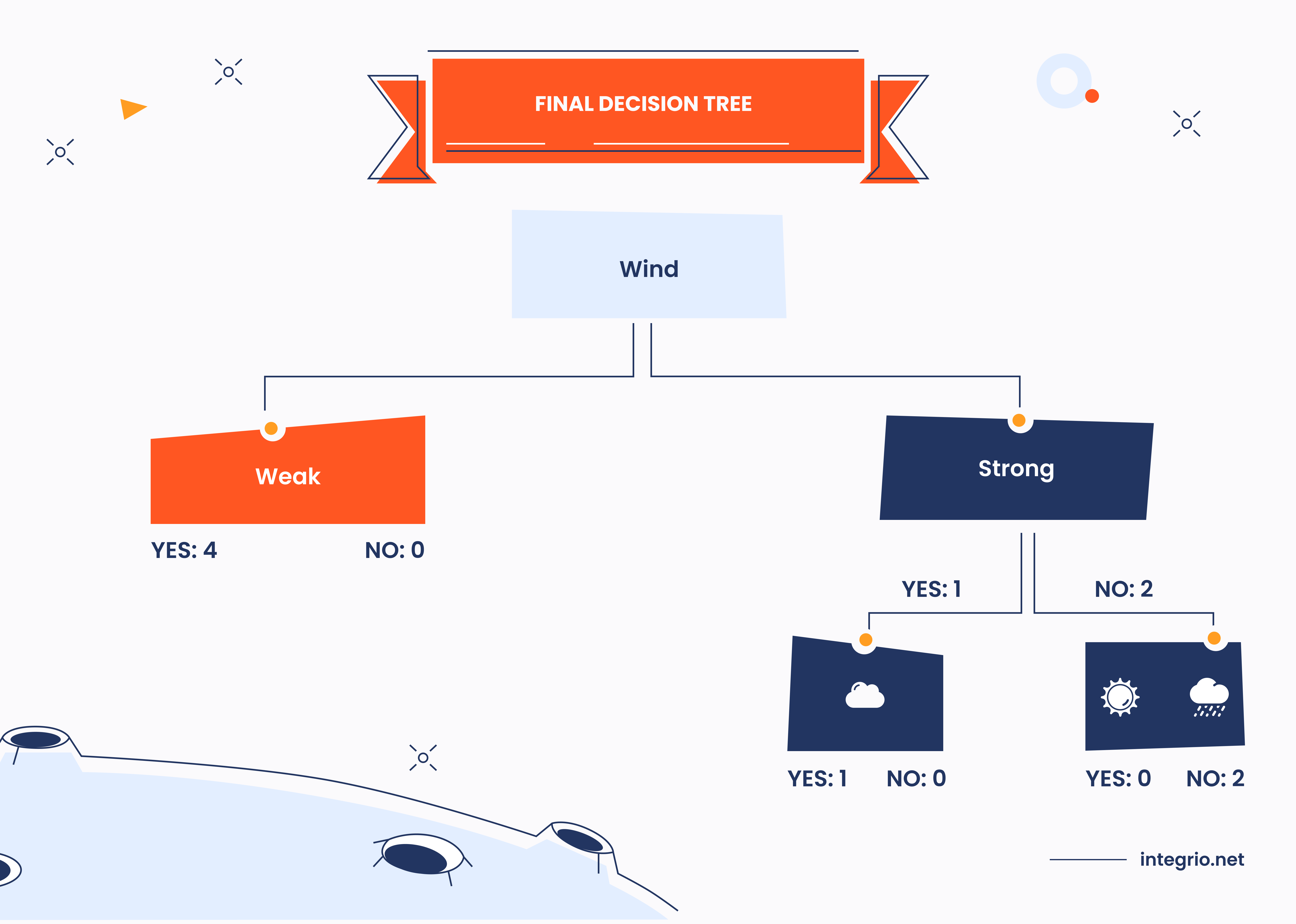
Since Wind feature is chosen as the root node, we need to continue building our decision tree. As it is seen from the tables above, Weak value creates the pure leaf with four Yes and zero No samples.

But the remaining Strong node is impure: single Yes and two No samples suggest that the road to purity has not beed finished yet. By picking other two features, namely Weather and Temp we should decide which one is better for prediction. Fortunately, this step is almost the same as before: we filter samples where Wind feature equals Strong, then for each feature (Weather, Temp) we create the candidate leaves, compute Gini index and weighted Gini values and compare them. These results are shown in the table below.

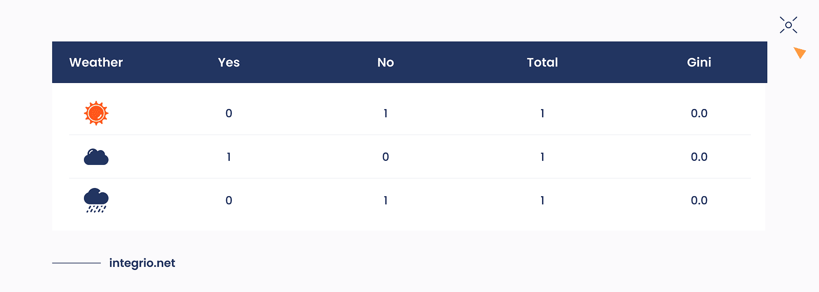
Weighted Gini = (1/3)*0 + (1/3)0 + (1/3)0 = 0.0 which signifies a perfect purity for all branches.

As we can see, the Weather leaf has smaller Gini value, so we should pick it to produce the final predictive layer. But here is the problem: this feature has three values while pure CART support only the binary nodes. To resolve this issue, CART will compare three possible partitions:

• Left: {Sunny} → No

  Right: {Cloudy, Rainy} → Yes, No → mixed

• Left: {Cloudy} → Yes

  Right: {Sunny, Rainy} → No, No → pure

• Left: {Rainy} → No

  Right: {Sunny, Cloudy} → No, Yes → mixed

The best partition in the second one with the lowest Gini index equals to 0. Even though there are three categories (Sunny, Cloudy, Rainy), CART finds a binary grouping that yields pure leaves. And that's it, our binary classification tree is completed. But what about Temp? In our small example,temperature will not appear in the CART tree. This is due to the fact that the categorical feature Weather already produces perfect purity at the node, so Temp provides no better split. So CART did not include this feature in the final tree.

Mechanics of Prunning

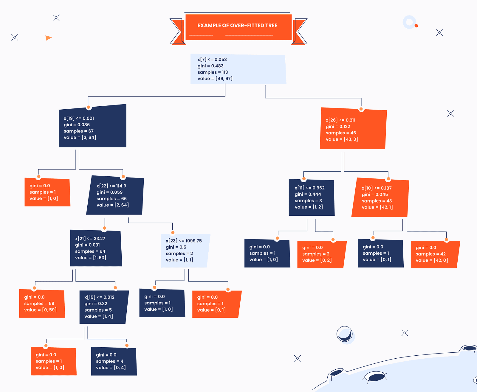
Before we dive into more advanced concepts, let's revise the over-fitting problem. Overfitting happens when a decision tree becomes too complex and learns not only the true patterns in the training data, but also random noise, outliers, and fluctuations that do not generalize to new data.

Decision trees keep splitting the data into smaller and purer subsets. Actually, decision tree ideally fits the training dataset. If not restricted, they may continue splitting until:

• Each leaf contains very few samples (even 1)
• The tree memorizes the dataset
• It starts capturing noise instead of patterns

A highly overfitted tree usually looks deep and bushy, with many branches/leaves. Thus, they can perform quiet poor on the unseen data.

Source: https://www.geeksforgeeks.org/machine-learning/pruning-decision-trees/

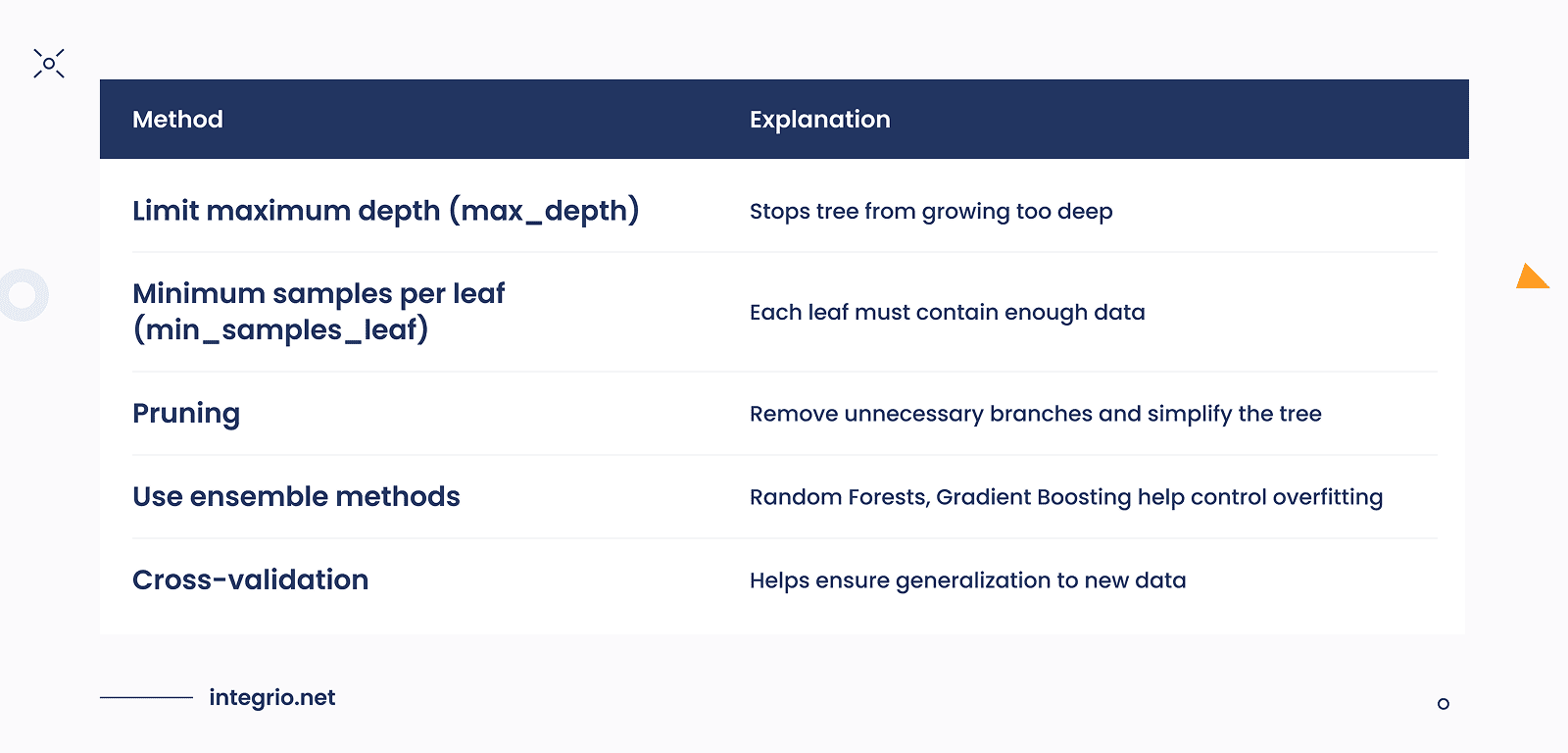
There are variety of methods how to deal with such issue (see table below). One of the effective approaches is called prunning. Pruning in CART is the process of cutting back (removing) parts of a fully grown decision tree to prevent overfitting and improve its performance on unseen data. CART (Breiman et al., 1984) uses a very specific and famous pruning method called Cost-Complexity Pruning.

The goal of Cost-Complexity Pruning or weakest link pruning is to reduce overfitting by making the decision tree smaller, without losing too much accuracy. In this algorithm, we have two important quantities:

R(T) = sum of errors (impurities) at all leaves of the tree, and |T| = number of leaf nodes in the tree.

A fully grown tree usually has low R(T), which signifies great training accuracy, and large |T|, which describes high complexity of the tree. Such characteristics usually point to the risk of overfitting.

For a single node i treated as a leaf, we compute its error as:

R(i) = Gini(i) * Number of Samples in i

Then, for the sub-tree T_i rooted at i:

To balance accuracy and simplicity, CART adds a penalty for the size of the tree:

R_α(T) = R(T) + α|T|,

where α ≥ 0 specifies how strongly we penalize complexity: higher α favors smaller trees.

To decide whether this simplification is worthwhile, CART evaluates how costly it is to keep the sub-tree instead of pruning it.

When considering pruning a subtree T_i rooted at node i, we define:

This cost is quantified by the cost–complexity measure:

where:

i is a root node considered as a single leaf (collapsed subtree);
T_i is the full subtree rooted at node i;
|T_i| is the number of leaves in that subtree;
R(T_i) is the total error (impurity) of that subtree;
R(i) is the error if the subtree is replaced by a single leaf i.

If α(t) is small, pruning this subtree increases error only slightly per leaf removed — it is a good candidate for pruning. Otherwise, pruning would cause a large increase in error, so we should keep it.

Therefore, pruning it results in a simpler tree with minimal sacrifice in accuracy.

The CART pruning algorithm does not prune everything at once. Instead, it repeats the following process gradually:

• Compute α(i) for all internal nodes (subtree roots)
• Prune the subtree with the smallest α(i) — the weakest branch. This produces a new tree with fewer leaves
• Update the tree and recompute α(i)
• Repeat until the tree is pruned to a single root or desired complexity
• Select the optimal subtree using a cross-validation dataset to choose the best α

Cost-complexity pruning systematically balances accuracy and simplicity, producing trees that generalize better to unseen data. By iteratively removing the weakest branches, we reduce overfitting while retaining the most informative structure, resulting in a robust, interpretable decision tree model.

Code Example

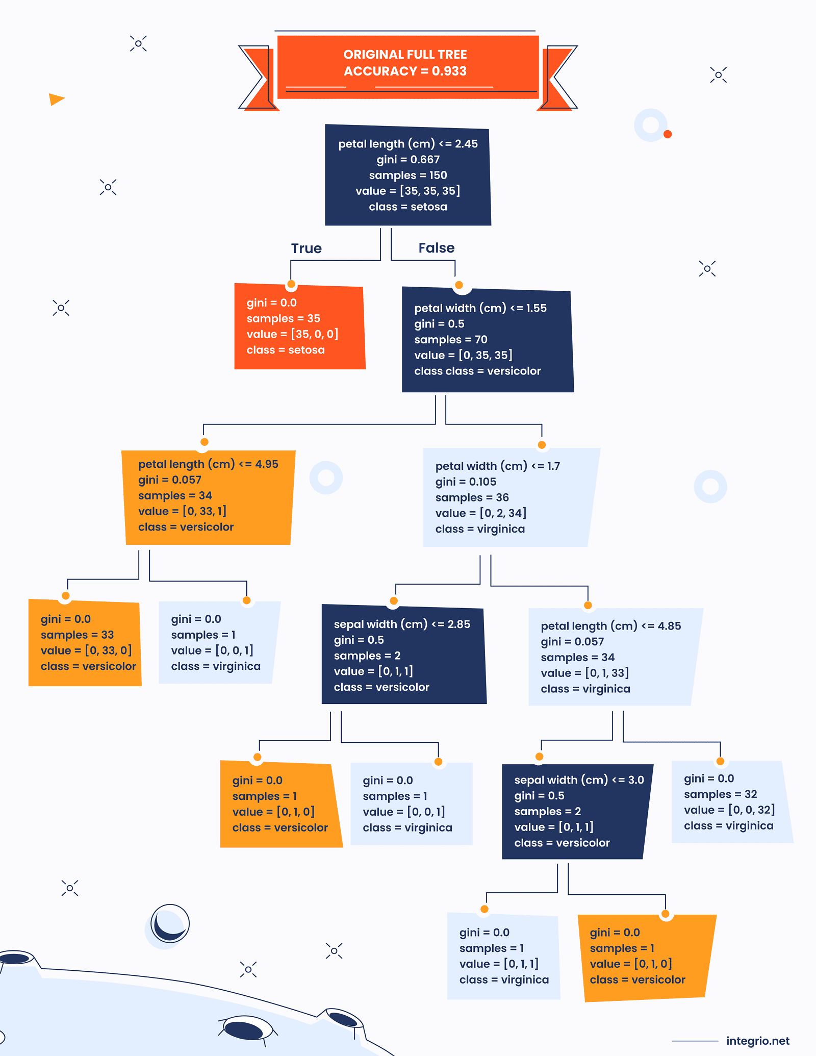
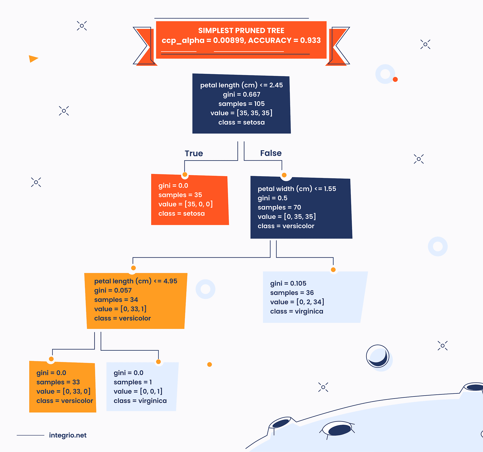
Below is the example of prunning mechanics for standard IRIS dataset.

Here, we compute test accuracy for each alpha along the pruning path. Then, we find all trees whose accuracy is within 1% of the best test accuracy. Afther this step, we pick largest alpha among them, giving the simplest tree that still performs well.

import numpy as np
import matplotlib.pyplot as plt
from sklearn.datasets import load_iris
from sklearn.model_selection import train_test_split, GridSearchCV
from sklearn.tree import DecisionTreeClassifier, plot_tree
from sklearn.metrics import accuracy_score

iris = load_iris()
X, y = iris.data, iris.target

X_train, X_test, y_train, y_test = train_test_split(
    X, y, test_size=0.3, random_state=42, stratify=y
)

test_acc = []
for alpha in ccp_alphas:
    clf = DecisionTreeClassifier(random_state=42, ccp_alpha=alpha)
    clf.fit(X_train, y_train)
    test_acc.append(accuracy_score(y_test, clf.predict(X_test)))

test_acc = np.array(test_acc)
best_acc = test_acc.max()
tolerance = 0.01

acceptable_alphas = ccp_alphas[test_acc >= best_acc - tolerance]
best_simple_alpha = acceptable_alphas.max()  # largest alpha = simplest tree

print(f"Best alpha for simplest tree within tolerance: {best_simple_alpha:.5f}")

tree_simple = DecisionTreeClassifier(random_state=42, ccp_alpha=best_simple_alpha)
tree_simple.fit(X_train, y_train)

acc_simple = accuracy_score(y_test, tree_simple.predict(X_test))
print(f"Accuracy of simplest pruned tree: {acc_simple:.3f}")

plt.figure(figsize=(20,8))

plt.subplot(1,2,1)
plot_tree(
    tree_full,
    feature_names=iris.feature_names,
    class_names=iris.target_names,
    filled=True, rounded=True
)
plt.title(f"Original Full Tree\nAccuracy={acc_full:.3f}")

plt.subplot(1,2,2)
plot_tree(
    tree_simple,
    feature_names=iris.feature_names,
    class_names=iris.target_names,
    filled=True, rounded=True
)
plt.title(f"Simplest Pruned Tree\nccp_alpha={best_simple_alpha:.5f}, Accuracy={acc_simple:.3f}")

plt.show()

Best alpha for simplest tree within tolerance: 0.00899
Accuracy of simplest pruned tree: 0.933
        

Feature Importance

Decision trees work by splitting the data using features to reduce impurity (Gini, entropy, etc.). So, a feature is considered important if it reduces impurity a lot and/or it is used often near the top of the tree. Feature importance measures how much each feature contributed to building the tree.

To formalize the definition, let's consider some feature f₁ which appears at k splits. So, its importance is calculated as follows:

Here, N_L,i is the number of samples in left nodes L at i-th split, N_R,i is the number of samples in right nodes R at i-th split, N_i is the number of samples in the parent node at i-th split. The importance score for each feature should be normalized in order to make feature importances comparable across all of them such that their sum equals 1:

where M is the total number of features.

Conclusion

In the materials we've shared so far, we've explored the basics of CART trees. But there's still a lot more to uncover! For example, we haven't yet dived into regression trees. We also haven't touched on concepts like gain ratio, entropy, the challenge of high variance, or advanced tree variants such as C4.5. Don't worry — we'll be covering all of these topics in our upcoming posts, so stay tuned!

FAQ